To handle the increasing variety and complexity of managerial forecasting problems, many forecasting techniques have been developed in recent years. Each has its special use, and care must be taken to select the correct technique for a particular application. The manager as well as the forecaster has a role to play in technique selection; and the better they understand the range of forecasting possibilities, the more likely it is that a company’s forecasting efforts will bear fruit.

The selection of a method depends on many factors—the context of the forecast, the relevance and availability of historical data, the degree of accuracy desirable, the time period to be forecast, the cost/ benefit (or value ) of the forecast to the company, and the time available for making the analysis.

These factors must be weighed constantly, and on a variety of levels. In general, for example, the forecaster should choose a technique that makes the best use of available data. If the forecaster can readily apply one technique of acceptable accuracy, he or she should not try to “gold plate” by using a more advanced technique that offers potentially greater accuracy but that requires nonexistent information or information that is costly to obtain. This kind of trade-off is relatively easy to make, but others, as we shall see, require considerably more thought.

Furthermore, where a company wishes to forecast with reference to a particular product, it must consider the stage of the product’s life cycle for which it is making the forecast . The availability of data and the possibility of establishing relationships between the factors depend directly on the maturity of a product, and hence the life-cycle stage is a prime determinant of the forecasting method to be used.

Our purpose here is to present an overview of this field by discussing the way a company ought to approach a forecasting problem, describing the methods available, and explaining how to match method to problem. We shall illustrate the use of the various techniques from our experience with them at Corning, and then close with our own forecast for the future of forecasting.

Although we believe forecasting is still an art, we think that some of the principles which we have learned through experience may be helpful to others.

Manager, Forecaster & Choice of Methods

A manager generally assumes that when asking a forecaster to prepare a specific projection, the request itself provides sufficient information for the forecaster to go to work and do the job. This is almost never true.

Successful forecasting begins with a collaboration between the manager and the forecaster, in which they work out answers to the following questions.

1. What is the purpose of the forecast—how is it to be used? This determines the accuracy and power required of the techniques, and hence governs selection. Deciding whether to enter a business may require only a rather gross estimate of the size of the market, whereas a forecast made for budgeting purposes should be quite accurate. The appropriate techniques differ accordingly.

Again, if the forecast is to set a “standard” against which to evaluate performance, the forecasting method should not take into account special actions, such as promotions and other marketing devices, since these are meant to change historical patterns and relationships and hence form part of the “performance” to be evaluated.

Forecasts that simply sketch what the future will be like if a company makes no significant changes in tactics and strategy are usually not good enough for planning purposes. On the other hand, if management wants a forecast of the effect that a certain marketing strategy under debate will have on sales growth, then the technique must be sophisticated enough to take explicit account of the special actions and events the strategy entails.

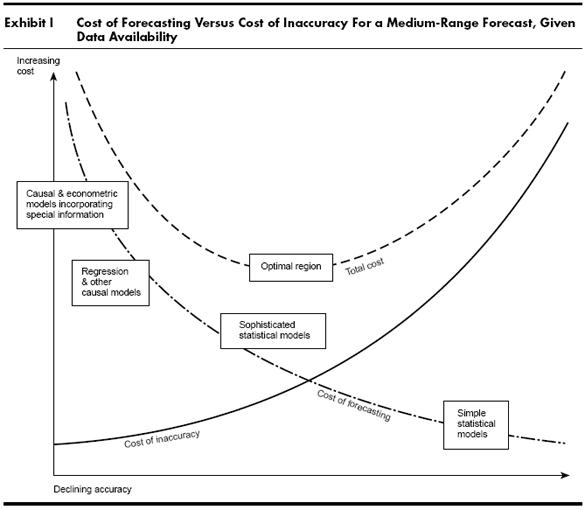
Techniques vary in their costs, as well as in scope and accuracy. The manager must fix the level of inaccuracy he or she can tolerate—in other words, decide how his or her decision will vary, depending on the range of accuracy of the forecast. This allows the forecaster to trade off cost against the value of accuracy in choosing a technique.

For example, in production and inventory control, increased accuracy is likely to lead to lower safety stocks. Here the manager and forecaster must weigh the cost of a more sophisticated and more expensive technique against potential savings in inventory costs.

Exhibit I shows how cost and accuracy increase with sophistication and charts this against the corresponding cost of forecasting errors, given some general assumptions. The most sophisticated technique that can be economically justified is one that falls in the region where the sum of the two costs is minimal.

Once the manager has defined the purpose of the forecast, the forecaster can advise the manager on how often it could usefully be produced. From a strategic point of view, they should discuss whether the decision to be made on the basis of the forecast can be changed later, if they find the forecast was inaccurate. If it can be changed, they should then discuss the usefulness of installing a system to track the accuracy of the forecast and the kind of tracking system that is appropriate.

2. What are the dynamics and components of the system for which the forecast will be made? This clarifies the relationships of interacting variables. Generally, the manager and the forecaster must review a flow chart that shows the relative positions of the different elements of the distribution system, sales system, production system, or whatever is being studied.

Exhibit II displays these elements for the system through which CGW’s major component for color TV sets—the bulb—flows to the consumer. Note the points where inventories are required or maintained in this manufacturing and distribution system—these are the pipeline elements, which exert important effects throughout the flow system and hence are of critical interest to the forecaster.

All the elements in dark gray directly affect forecasting procedure to some extent, and the color key suggests the nature of CGW’s data at each point, again a prime determinant of technique selection since different techniques require different kinds of inputs. Where data are unavailable or costly to obtain, the range of forecasting choices is limited.

The flow chart should also show which parts of the system are under the control of the company doing the forecasting. In Exhibit II, this is merely the volume of glass panels and funnels supplied by Corning to the tube manufacturers.

In the part of the system where the company has total control, management tends to be tuned in to the various cause-and-effect relationships, and hence can frequently use forecasting techniques that take causal factors explicitly into account.

The flow chart has special value for the forecaster where causal prediction methods are called for because it enables him or her to conjecture about the possible variations in sales levels caused by inventories and the like, and to determine which factors must be considered by the technique to provide the executive with a forecast of acceptable accuracy.

Once these factors and their relationships have been clarified, the forecaster can build a causal model of the system which captures both the facts and the logic of the situation—which is, after all, the basis of sophisticated forecasting.

3. How important is the past in estimating the future? Significant changes in the system—new products, new competitive strategies, and so forth—diminish the similarity of past and future. Over the short term, recent changes are unlikely to cause overall patterns to alter, but over the long term their effects are likely to increase. The executive and the forecaster must discuss these fully.

Three General Types

Once the manager and the forecaster have formulated their problem, the forecaster will be in a position to choose a method.

There are three basic types— qualitative techniques, time series analysis and projection, and causal models . The first uses qualitative data (expert opinion, for example) and information about special events of the kind already mentioned, and may or may not take the past into consideration.

The second, on the other hand, focuses entirely on patterns and pattern changes, and thus relies entirely on historical data.

The third uses highly refined and specific information about relationships between system elements, and is powerful enough to take special events formally into account. As with time series analysis and projection techniques, the past is important to causal models.

These differences imply (quite correctly) that the same type of forecasting technique is not appropriate to forecast sales, say, at all stages of the life cycle of a product—for example, a technique that relies on historical data would not be useful in forecasting the future of a totally new product that has no history.

The major part of the balance of this article will be concerned with the problem of suiting the technique to the life-cycle stages. We hope to give the executive insight into the potential of forecasting by showing how this problem is to be approached. But before we discuss the life cycle, we need to sketch the general functions of the three basic types of techniques in a bit more detail.

Qualitative techniques

Primarily, these are used when data are scarce—for example, when a product is first introduced into a market. They use human judgment and rating schemes to turn qualitative information into quantitative estimates.

The objective here is to bring together in a logical, unbiased, and systematic way all information and judgments which relate to the factors being estimated. Such techniques are frequently used in new-technology areas, where development of a product idea may require several “inventions,” so that R&D demands are difficult to estimate, and where market acceptance and penetration rates are highly uncertain.

The multi-page chart “Basic Forecasting Techniques” presents several examples of this type (see the first section), including market research and the now-familiar Delphi technique. 1 In this chart we have tried to provide a body of basic information about the main kinds of forecasting techniques. Some of the techniques listed are not in reality a single method or model, but a whole family. Thus our statements may not accurately describe all the variations of a technique and should rather be interpreted as descriptive of the basic concept of each.

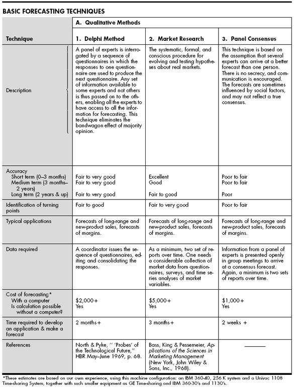
A disclaimer about estimates in the chart is also in order. Estimates of costs are approximate, as are computation times, accuracy ratings, and ratings for turning-point identification. The costs of some procedures depend on whether they are being used routinely or are set up for a single forecast; also, if weightings or seasonals have to be determined anew each time a forecast is made, costs increase significantly. Still, the figures we present may serve as general guidelines.

The reader may find frequent reference to this gate-fold helpful for the remainder of the article.

Time series analysis

These are statistical techniques used when several years’ data for a product or product line are available and when relationships and trends are both clear and relatively stable.

One of the basic principles of statistical forecasting—indeed, of all forecasting when historical data are available—is that the forecaster should use the data on past performance to get a “speedometer reading” of the current rate (of sales, say) and of how fast this rate is increasing or decreasing. The current rate and changes in the rate—“acceleration” and “deceleration”—constitute the basis of forecasting. Once they are known, various mathematical techniques can develop projections from them.

The matter is not so simple as it sounds, however. It is usually difficult to make projections from raw data since the rates and trends are not immediately obvious; they are mixed up with seasonal variations, for example, and perhaps distorted by such factors as the effects of a large sales promotion campaign. The raw data must be massaged before they are usable, and this is frequently done by time series analysis.

Now, a time series is a set of chronologically ordered points of raw data—for example, a division’s sales of a given product, by month, for several years. Time series analysis helps to identify and explain:

Any regularity or systematic variation in the series of data which is due to seasonality—the “seasonals.”

Cyclical patterns that repeat any two or three years or more.

Trends in the data.

Growth rates of these trends.

(Unfortunately, most existing methods identify only the seasonals, the combined effect of trends and cycles, and the irregular, or chance, component. That is, they do not separate trends from cycles . We shall return to this point when we discuss time series analysis in the final stages of product maturity.)

Once the analysis is complete, the work of projecting future sales (or whatever) can begin.

We should note that while we have separated analysis from projection here for purposes of explanation, most statistical forecasting techniques actually combine both functions in a single operation.

A future like the past:

It is obvious from this description that all statistical techniques are based on the assumption that existing patterns will continue into the future. This assumption is more likely to be correct over the short term than it is over the long term, and for this reason these techniques provide us with reasonably accurate forecasts for the immediate future but do quite poorly further into the future (unless the data patterns are extraordinarily stable).

For this same reason, these techniques ordinarily cannot predict when the rate of growth in a trend will change significantly—for example, when a period of slow growth in sales will suddenly change to a period of rapid decay.

Such points are called turning points . They are naturally of the greatest consequence to the manager, and, as we shall see, the forecaster must use different tools from pure statistical techniques to predict when they will occur.

Causal models

When historical data are available and enough analysis has been performed to spell out explicitly the relationships between the factor to be forecast and other factors (such as related businesses, economic forces, and socioeconomic factors), the forecaster often constructs a causal model .

A causal model is the most sophisticated kind of forecasting tool. It expresses mathematically the relevant causal relationships, and may include pipeline considerations (i.e., inventories) and market survey information. It may also directly incorporate the results of a time series analysis.

The causal model takes into account everything known of the dynamics of the flow system and utilizes predictions of related events such as competitive actions, strikes, and promotions. If the data are available, the model generally includes factors for each location in the flow chart (as illustrated in Exhibit II) and connects these by equations to describe overall product flow.

If certain kinds of data are lacking, initially it may be necessary to make assumptions about some of the relationships and then track what is happening to determine if the assumptions are true. Typically, a causal model is continually revised as more knowledge about the system becomes available.

Again, see the gatefold for a rundown on the most common types of causal techniques. As the chart shows, causal models are by far the best for predicting turning points and preparing long-range forecasts.

Methods, Products & the Life Cycle

At each stage of the life of a product, from conception to steady-state sales, the decisions that management must make are characteristically quite different, and they require different kinds of information as a base. The forecasting techniques that provide these sets of information differ analogously. Exhibit III summarizes the life stages of a product, the typical decisions made at each, and the main forecasting techniques suitable at each.

Equally, different products may require different kinds of forecasting. Two CGW products that have been handled quite differently are the major glass components for color TV tubes, of which Corning is a prime supplier, and Corning Ware cookware, a proprietary consumer product line. We shall trace the forecasting methods used at each of the four different stages of maturity of these products to give some firsthand insight into the choice and application of some of the major techniques available today.

Before we begin, let us note how the situations differ for the two kinds of products:

For a consumer product like the cookware, the manufacturer’s control of the distribution pipeline extends at least through the distributor level. Thus the manufacturer can effect or control consumer sales quite directly, as well as directly control some of the pipeline elements.

Many of the changes in shipment rates and in overall profitability are therefore due to actions taken by manufacturers themselves. Tactical decisions on promotions, specials, and pricing are usually at their discretion as well. The technique selected by the forecaster for projecting sales therefore should permit incorporation of such “special information.” One may have to start with simple techniques and work up to more sophisticated ones that embrace such possibilities, but the final goal is there.

Where the manager’s company supplies a component to an OEM, as Corning does for tube manufacturers, the company does not have such direct influence or control over either the pipeline elements or final consumer sales. It may be impossible for the company to obtain good information about what is taking place at points further along the flow system (as in the upper segment of Exhibit II), and, in consequence, the forecaster will necessarily be using a different genre of forecasting from what is used for a consumer product.

Between these two examples, our discussion will embrace nearly the whole range of forecasting techniques. As necessary, however, we shall touch on other products and other forecasting methods.

1. Product Development

In the early stages of product development, the manager wants answers to questions such as these:

What are the alternative growth opportunities to pursuing product X ?

How have established products similar to X fared?

Should we enter this business; and if so, in what segments?

How should we allocate R&D efforts and funds?

How successful will different product concepts be?

How will product X fit into the markets five or ten years from now?

Forecasts that help to answer these long-range questions must necessarily have long horizons themselves.

A common objection to much long-range forecasting is that it is virtually impossible to predict with accuracy what will happen several years into the future. We agree that uncertainty increases when a forecast is made for a period more than two years out. However, at the very least, the forecast and a measure of its accuracy enable the manager to know the risks in pursuing a selected strategy and in this knowledge to choose an appropriate strategy from those available.

Systematic market research is, of course, a mainstay in this area. For example, priority pattern analysis can describe consumers’ preferences and the likelihood they will buy a product, and thus is of great value in forecasting (and updating) penetration levels and rates. But there are other tools as well, depending on the state of the market and the product concept.

For a defined market

While there can be no direct data about a product that is still a gleam in the eye, information about its likely performance can be gathered in a number of ways, provided the market in which it is to be sold is a known entity.

First, one can compare a proposed product with competitors’ present and planned products, ranking it on quantitative scales for different factors. We call this product differences measurement . 2

If this approach is to be successful, it is essential that the (in-house) experts who provide the basic data come from different disciplines—marketing, R&D, manufacturing, legal, and so on—and that their opinions be unbiased.

Second, and more formalistically, one can construct disaggregate market models by separating off different segments of a complex market for individual study and consideration. Specifically, it is often useful to project the S -shaped growth curves for the levels of income of different geographical regions.

When color TV bulbs were proposed as a product, CGW was able to identify the factors that would influence sales growth. Then, by disaggregating consumer demand and making certain assumptions about these factors, it was possible to develop an S -curve for rate of penetration of the household market that proved most useful to us.

Third, one can compare a projected product with an “ancestor” that has similar characteristics. In 1965, we disaggregated the market for color television by income levels and geographical regions and compared these submarkets with the historical pattern of black-and-white TV market growth. We justified this procedure by arguing that color TV represented an advance over black-and-white analogous to (although less intense than) the advance that black-and-white TV represented over radio. The analyses of black-and-white TV market growth also enabled us to estimate the variability to be expected—that is, the degree to which our projections would differ from actual as the result of economic and other factors.

The prices of black-and-white TV and other major household appliances in 1949, consumer disposable income in 1949, the prices of color TV and other appliances in 1965, and consumer disposable income for 1965 were all profitably considered in developing our long-range forecast for color-TV penetration on a national basis. The success patterns of black-and-white TV, then, provided insight into the likelihood of success and sales potential of color TV.

Our predictions of consumer acceptance of Corning Ware cookware, on the other hand, were derived primarily from one expert source, a manager who thoroughly understood consumer preferences and the housewares market. These predictions have been well borne out. This reinforces our belief that sales forecasts for a new product that will compete in an existing market are bound to be incomplete and uncertain unless one culls the best judgments of fully experienced personnel.

For an undefined market

Frequently, however, the market for a new product is weakly defined or few data are available, the product concept is still fluid, and history seems irrelevant. This is the case for gas turbines, electric and steam automobiles, modular housing, pollution measurement devices, and time-shared computer terminals.

Many organizations have applied the Delphi method of soliciting and consolidating experts’ opinions under these circumstances. At CGW, in several instances, we have used it to estimate demand for such new products, with success.

Input-output analysis, combined with other techniques, can be extremely useful in projecting the future course of broad technologies and broad changes in the economy. The basic tools here are the input-output tables of U.S. industry for 1947, 1958, and 1963, and various updatings of the 1963 tables prepared by a number of groups who wished to extrapolate the 1963 figures or to make forecasts for later years.

Since a business or product line may represent only a small sector of an industry, it may be difficult to use the tables directly. However, a number of companies are disaggregating industries to evaluate their sales potential and to forecast changes in product mixes—the phasing out of old lines and introduction of others. For example, Quantum-Science Corporation (MAPTEK) has developed techniques that make input-output analyses more directly useful to people in the electronics business today. (Other techniques, such as panel consensus and visionary forecasting, seem less effective to us, and we cannot evaluate them from our own experience.)

2. Testing & Introduction

Before a product can enter its (hopefully) rapid penetration stage, the market potential must be tested out and the product must be introduced—and then more market testing may be advisable. At this stage, management needs answers to these questions:

What shall our marketing plan be—which markets should we enter and with what production quantities?

How much manufacturing capacity will the early production stages require?

As demand grows, where should we build this capacity?

How shall we allocate our R&D resources over time?

Significant profits depend on finding the right answers, and it is therefore economically feasible to expend relatively large amounts of effort and money on obtaining good forecasts, short-, medium-, and long-range.

A sales forecast at this stage should provide three points of information: the date when rapid sales will begin, the rate of market penetration during the rapid-sales stage, and the ultimate level of penetration, or sales rate, during the steady-state stage.

Using early data

The date when a product will enter the rapid-growth stage is hard to predict three or four years in advance (the usual horizon). A company’s only recourse is to use statistical tracking methods to check on how successfully the product is being introduced, along with routine market studies to determine when there has been a significant increase in the sales rate.

Furthermore, the greatest care should be taken in analyzing the early sales data that start to accumulate once the product has been introduced into the market. For example, it is important to distinguish between sales to innovators, who will try anything new, and sales to imitators, who will buy a product only after it has been accepted by innovators, for it is the latter group that provides demand stability. Many new products have initially appeared successful because of purchases by innovators, only to fail later in the stretch.

Tracking the two groups means market research, possibly via opinion panels. A panel ought to contain both innovators and imitators, since innovators can teach one a lot about how to improve a product while imitators provide insight into the desires and expectations of the whole market.

The color TV set, for example, was introduced in 1954, but did not gain acceptance from the majority of consumers until late 1964. To be sure, the color TV set could not leave the introduction stage and enter the rapid-growth stage until the networks had substantially increased their color programming. However, special flag signals like “substantially increased network color programming” are likely to come after the fact, from the planning viewpoint; and in general, we find, scientifically designed consumer surveys conducted on a regular basis provide the earliest means of detecting turning points in the demand for a product.

Similar-product technique

Although statistical tracking is a useful tool during the early introduction stages, there are rarely sufficient data for statistical forecasting. Market research studies can naturally be useful, as we have indicated. But, more commonly, the forecaster tries to identify a similar, older product whose penetration pattern should be similar to that of the new product, since overall markets can and do exhibit consistent patterns.

Again, let’s consider color television and the forecasts we prepared in 1965.

For the year 1947–1968, Exhibit IV shows total consumer expenditures, appliance expenditures, expenditures for radios and TVs, and relevant percentages. Column 4 shows that total expenditures for appliances are relatively stable over periods of several years; hence, new appliances must compete with existing ones, especially during recessions (note the figures for 1948–1949, 1953–1954, 1957–1958, and 1960–1961).

Certain special fluctuations in these figures are of special significance here. When black-and-white TV was introduced as a new product in 1948–1951, the ratio of expenditures on radio and TV sets to total expenditures for consumer goods (see column 7) increased about 33 % (from 1.23 % to 1.63 % ), as against a modest increase of only 13 % (from 1.63 % to 1.88 % ) in the ratio for the next decade. (A similar increase of 33 % occurred in 1962–1966 as color TV made its major penetration.)

Probably the acceptance of black-and-white TV as a major appliance in 1950 caused the ratio of all major household appliances to total consumer goods (see column 5) to rise to 4.98 % ; in other words, the innovation of TV caused the consumer to start spending more money on major appliances around 1950.

Our expectation in mid-1965 was that the introduction of color TV would induce a similar increase. Thus, although this product comparison did not provide us with an accurate or detailed forecast, it did place an upper bound on the future total sales we could expect.

The next step was to look at the cumulative penetration curve for black-and-white TVs in U.S. households, shown in Exhibit V. We assumed color-TV penetration would have a similar S -curve, but that it would take longer for color sets to penetrate the whole market (that is, reach steady-state sales). Whereas it took black-and-white TV 10 years to reach steady state, qualitative expert-opinion studies indicated that it would take color twice that long—hence the more gradual slope of the color-TV curve.

At the same time, studies conducted in 1964 and 1965 showed significantly different penetration sales for color TV in various income groups, rates that were helpful to us in projecting the color-TV curve and tracking the accuracy of our projection.

With these data and assumptions, we forecast retail sales for the remainder of 1965 through mid-1970 (see the dotted section of the lower curve in Exhibit V). The forecasts were accurate through 1966 but too high in the following three years, primarily because of declining general economic conditions and changing pricing policies

We should note that when we developed these forecasts and techniques, we recognized that additional techniques would be necessary at later times to maintain the accuracy that would be needed in subsequent periods. These forecasts provided acceptable accuracy for the time they were made, however, since the major goal then was only to estimate the penetration rate and the ultimate, steady-state level of sales. Making refined estimates of how the manufacturing-distribution pipelines will behave is an activity that properly belongs to the next life-cycle stage.

Other approaches:

When it is not possible to identify a similar product, as was the case with CGW’s self-cleaning oven and flat-top cooking range (Counterange), another approach must be used.

For the purposes of initial introduction into the markets, it may only be necessary to determine the minimum sales rate required for a product venture to meet corporate objectives. Analyses like input-output, historical trend, and technological forecasting can be used to estimate this minimum. Also, the feasibility of not entering the market at all, or of continuing R&D right up to the rapid-growth stage, can best be determined by sensitivity analysis.

Predicting rapid growth

To estimate the date by which a product will enter the rapid-growth stage is another matter. As we have seen, this date is a function of many factors: the existence of a distribution system, customer acceptance of or familiarity with the product concept, the need met by the product, significant events (such as color network programming), and so on.

As well as by reviewing the behavior of similar products, the date may be estimated through Delphi exercises or through rating and ranking schemes, whereby the factors important to customer acceptance are estimated, each competitor product is rated on each factor, and an overall score is tallied for the competitor against a score for the new product.

As we have said, it is usually difficult to forecast precisely when the turning point will occur; and, in our experience, the best accuracy that can be expected is within three months to two years of the actual time.

It is occasionally true, of course, that one can be certain a new product will be enthusiastically accepted. Market tests and initial customer reaction made it clear there would be a large market for Corning Ware cookware. Since the distribution system was already in existence, the time required for the line to reach rapid growth depended primarily on our ability to manufacture it. Sometimes forecasting is merely a matter of calculating the company’s capacity—but not ordinarily.

3. Rapid Growth

When a product enters this stage, the most important decisions relate to facilities expansion. These decisions generally involve the largest expenditures in the cycle (excepting major R&D decisions), and commensurate forecasting and tracking efforts are justified.

Forecasting and tracking must provide the executive with three kinds of data at this juncture:

Firm verification of the rapid-growth rate forecast made previously.

A hard date when sales will level to “normal,” steady-state growth .

For component products, the deviation in the growth curve that may be caused by characteristic conditions along the pipeline —for example, inventory blockages.

Forecasting the growth rate

Medium- and long-range forecasting of the market growth rate and of the attainment of steady-state sales requires the same measures as does the product introduction stage—detailed marketing studies (especially intention-to-buy surveys) and product comparisons.

When a product has entered rapid growth, on the other hand, there are generally sufficient data available to construct statistical and possibly even causal growth models (although the latter will necessarily contain assumptions that must be verified later).

We estimated the growth rate and steady-state rate of color TV by a crude econometric-marketing model from data available at the beginning of this stage. We conducted frequent marketing studies as well.

The growth rate for Corning Ware Cookware, as we explained, was limited primarily by our production capabilities; and hence the basic information to be predicted in that case was the date of leveling growth. Because substantial inventories buffered information on consumer sales all along the line, good field data were lacking, which made this date difficult to estimate. Eventually we found it necessary to establish a better (more direct) field information system.

As well as merely buffering information, in the case of a component product, the pipeline exerts certain distorting effects on the manufacturer’s demand; these effects, although highly important, are often illogically neglected in production or capacity planning.

Simulating the pipeline

While the ware-in-process demand in the pipeline has an S -curve like that of retail sales, it may lag or lead sales by several months, distorting the shape of the demand on the component supplier.

Exhibit VI shows the long-term trend of demand on a component supplier other than Corning as a function of distributor sales and distributor inventories. As one can see from this curve, supplier sales may grow relatively sharply for several months and peak before retail sales have leveled off. The implications of these curves for facilities planning and allocation are obvious.

Here we have used components for color TV sets for our illustration because we know from our own experience the importance of the long flow time for color TVs that results from the many sequential steps in manufacturing and distribution (recall Exhibit II). There are more spectacular examples; for instance, it is not uncommon for the flow time from component supplier to consumer to stretch out to two years in the case of truck engines.

To estimate total demand on CGW production, we used a retail demand model and a pipeline simulation. The model incorporated penetration rates, mortality curves, and the like. We combined the data generated by the model with market-share data, data on glass losses, and other information to make up the corpus of inputs for the pipeline simulation. The simulation output allowed us to apply projected curves like the ones shown in Exhibit VI to our own component-manufacturing planning.

Simulation is an excellent tool for these circumstances because it is essentially simpler than the alternative—namely, building a more formal, more “mathematical” model. That is, simulation bypasses the need for analytical solution techniques and for mathematical duplication of a complex environment and allows experimentation. Simulation also informs us how the pipeline elements will behave and interact over time—knowledge that is very useful in forecasting, especially in constructing formal causal models at a later date.

Tracking & warning

This knowledge is not absolutely “hard,” of course, and pipeline dynamics must be carefully tracked to determine if the various estimates and assumptions made were indeed correct. Statistical methods provide a good short-term basis for estimating and checking the growth rate and signaling when turning points will occur.

In late 1965 it appeared to us that the ware-in-process demand was increasing, since there was a consistent positive difference between actual TV bulb sales and forecasted bulb sales. Conversations with product managers and other personnel indicated there might have been a significant change in pipeline activity; it appeared that rapid increases in retail demand were boosting glass requirements for ware-in-process, which could create a hump in the S -curve like the one illustrated in Exhibit VI. This humping provided additional profit for CGW in 1966 but had an adverse effect in 1967. We were able to predict this hump, but unfortunately we were unable to reduce or avoid it because the pipeline was not sufficiently under our control.

The inventories all along the pipeline also follow an S -curve (as shown in Exhibit VI), a fact that creates and compounds two characteristic conditions in the pipeline as a whole: initial overfilling and subsequent shifts between too much and too little inventory at various points—a sequence of feast-and-famine conditions.

For example, the simpler distribution system for Corning Ware had an S -curve like the ones we have examined. When the retail sales slowed from rapid to normal growth, however, there were no early indications from shipment data that this crucial turning point had been reached. Data on distributor inventories gave us some warning that the pipeline was over filling, but the turning point at the retail level was still not identified quickly enough, as we have mentioned before, because of lack of good data at the level. We now monitor field information regularly to identify significant changes, and adjust our shipment forecasts accordingly.

Main concerns

One main activity during the rapid-growth stage, then, is to check earlier estimates and, if they appear incorrect, to compute as accurately as possible the error in the forecast and obtain a revised estimate.

In some instances, models developed earlier will include only “macroterms”; in such cases, market research can provide information needed to break these down into their components. For example, the color-TV forecasting model initially considered only total set penetrations at different income levels, without considering the way in which the sets were being used. Therefore, we conducted market surveys to determine set use more precisely.

Equally, during the rapid-growth stage, submodels of pipeline segments should be expanded to incorporate more detailed information as it is received. In the case of color TV, we found we were able to estimate the overall pipeline requirements for glass bulbs, the CGW market-share factors, and glass losses, and to postulate a probability distribution around the most likely estimates. Over time, it was easy to check these forecasts against actual volume of sales, and hence to check on the procedures by which we were generating them.

We also found we had to increase the number of factors in the simulation model—for instance, we had to expand the model to consider different sizes of bulbs—and this improved our overall accuracy and usefulness.

The preceding is only one approach that can be used in forecasting sales of new products that are in a rapid growth. Others have discussed different ones. 3

4. Steady State

The decisions the manager at this stage are quite different from those made earlier. Most of the facilities planning has been squared away, and trends and growth rates have become reasonably stable. It is possible that swings in demand and profit will occur because of changing economic conditions, new and competitive products, pipeline dynamics, and so on, and the manager will have to maintain the tracking activities and even introduce new ones. However, by and large, the manager will concentrate forecasting attention on these areas:

Long- and short-term production planning.

Setting standards to check the effectiveness of marketing strategies.

Projections designed to aid profit planning.

The manager will also need a good tracking and warning system to identify significantly declining demand for the product (but hopefully that is a long way off).

To be sure, the manager will want margin and profit projection and long-range forecasts to assist planning at the corporate level. However, short- and medium-term sales forecasts are basic to these more elaborate undertakings, and we shall concentrate on sales forecasts.

Adequate tools at hand

In planning production and establishing marketing strategy for the short and medium term, the manager’s first considerations are usually an accurate estimate of the present sales level and an accurate estimate of the rate at which this level is changing.

The forecaster thus is called on for two related contributions at this stage:

To provide estimates of trends and seasonals, which obviously affect the sales level. Seasonals are particularly important for both overall production planning and inventory control. To do this, the forecaster needs to apply time series analysis and projection techniques—that is, statistical techniques.

To relate the future sales level to factors that are more easily predictable, or have a “lead” relationship with sales, or both. To do this the forecaster needs to build causal models .

The type of product under scrutiny is very important in selecting the techniques to be used.

For Corning Ware, where the levels of the distribution system are organized in a relatively straightforward way, we use statistical methods to forecast shipments and field information to forecast changes in shipment rates. We are now in the process of incorporating special information—marketing strategies, economic forecasts, and so on—directly into the shipment forecasts. This is leading us in the direction of a causal forecasting model.

On the other hand, a component supplier may be able to forecast total sales with sufficient accuracy for broad-load production planning, but the pipeline environment may be so complex that the best recourse for short-term projections is to rely primarily on salespersons’ estimates. We find this true, for example, in estimating the demand for TV glass by size and customer. In such cases, the best role for statistical methods is providing guides and checks for salespersons’ forecasts.

In general, however, at this point in the life cycle, sufficient time series data are available and enough causal relationships are known from direct experience and market studies so that the forecaster can indeed apply these two powerful sets of tools. Historical data for at least the last several years should be available. The forecaster will use all of it, one way or another.

We might mention a common criticism at this point. People frequently object to using more than a few of the most recent data points (such as sales figures in the immediate past) for building projections, since, they say, the current situation is always so dynamic and conditions are changing so radically and quickly that historical data from further back in time have little or no value.

We think this point of view had little validity. A graph of several years’ sales data, such as the one shown in Part A of Exhibit VII, gives an impression of a sales trend one could not possibly get if one were to look only at two or three of the latest data points.

In practice, we find, overall patterns tend to continue for a minimum of one or two quarters into the future, even when special conditions cause sales to fluctuate for one or two (monthly) periods in the immediate future.

For short-term forecasting for one to three months ahead, the effects of such factors as general economic conditions are minimal, and do not cause radical shifts in demand patterns. And because trends tend to change gradually rather than suddenly, statistical and other quantitative methods are excellent for short-term forecasting. Using one or only a few of the most recent data points will result in giving insufficient consideration of the nature of trends, cycles, and seasonal fluctuations in sales.

Granting the applicability of the techniques, we must go on to explain how the forecaster identifies precisely what is happening when sales fluctuate from one period to the next and how such fluctuations can be forecast.

Sorting trends & seasonals

A trend and a seasonal are obviously two quite different things, and they must be handled separately in forecasting.

Consider what would happen, for example, if a forecaster were merely to take an average of the most recent data points along a curve, combine this with other, similar average points stretching backward into the immediate past, and use these as the basis for a projection. The forecaster might easily overreact to random changes, mistaking them for evidence of a prevailing trend, mistake a change in the growth rate for a seasonal, and so on.

To avoid precisely this sort of error, the moving average technique, which is similar to the hypothetical one just described, uses data points in such a way that the effects of seasonals (and irregularities) are eliminated.

Furthermore, the executive needs accurate estimates of trends and accurate estimates of seasonality to plan broad-load production, to determine marketing efforts and allocations, and to maintain proper inventories—that is, inventories that are adequate to customer demand but are not excessively costly.

Before going any further, it might be well to illustrate what such sorting-out looks like. Parts A, B, and C of Exhibit VII show the initial decomposition of raw data for factory sales of color TV sets between 1965 and mid-1970. Part A presents the raw data curve. Part B shows the seasonal factors that are implicit in the raw data—quite a consistent pattern, although there is some variation from year to year. (In the next section we shall explain where this graph of the seasonals comes from.)

Part C shows the result of discounting the raw data curve by the seasonals of Part B; this is the so-called deseasonalized data curve. Next, in Part D, we have drawn the smoothest or “best” curve possible through the deseasonalized curve, thereby obtaining the trend cycle . (We might further note that the differences between this trend-cycle line and the deseasonalized data curve represent the irregular or nonsystematic component that the forecaster must always tolerate and attempt to explain by other methods.)

In sum, then, the objective of the forecasting technique used here is to do the best possible job of sorting out trends and seasonalities. Unfortunately, most forecasting methods project by a smoothing process analogous to that of the moving average technique, or like that of the hypothetical technique we described at the beginning of this section, and separating trends and seasonals more precisely will require extra effort and cost.

Still, sorting-out approaches have proved themselves in practice. We can best explain the reasons for their success by roughly outlining the way we construct a sales forecast on the basis of trends, seasonals, and data derived from them. This is the method:

Graph the rate at which the trend is changing. For the illustration given in Exhibit VII, this graph is shown in Part E . This graph describes the successive ups and downs of the trend cycle shown in Part D .

Project this growth rate forward over the interval to be forecasted. Assuming we were forecasting back in mid-1970, we should be projecting into the summer months and possible into the early fall.

Add this growth rate (whether positive or negative) to the present sales rate. This might be called the unseasonalized sales rate.

Project the seasonals of Part B for the period in question, and multiply the unseasonalized forecasted rate by these seasonals. The product will be the forecasted sales rate, which is what we desired.

In special cases where there are no seasonals to be considered, of course, this process is much simplified, and fewer data and simpler techniques may be adequate.

We have found that an analysis of the patterns of change in the growth rate gives us more accuracy in predicting turning points (and therefore changes from positive to negative growth, and vice versa) than when we use only the trend cycle.

The main advantage of considering growth change, in fact, is that it is frequently possible to predict earlier when a no-growth situation will occur. The graph of change in growth thus provides an excellent visual base for forecasting and for identifying the turning point as well.

X-11 technique

The reader will be curious to know how one breaks the seasonals out of raw sales data and exactly how one derives the change-in-growth curve from the trend line.

One of the best techniques we know for analyzing historical data in depth to determine seasonals, present sales rate, and growth is the X-11 Census Bureau Technique, which simultaneously removes seasonals from raw information and fits a trend-cycle line to the data. It is very comprehensive: at a cost of about $ 10, it provides detailed information on seasonals, trends, the accuracy of the seasonals and the trend cycle fit, and a number of other measures. The output includes plots of the trend cycle and the growth rate, which can concurrently be received on graphic displays on a time-shared terminal.

Although the X-11 was not originally developed as a forecasting method, it does establish a base from which good forecasts can be made. One should note, however, that there is some instability in the trend line for the most recent data points, since the X-11, like virtually all statistical techniques, uses some form of moving average. It has therefore proved of value to study the changes in growth pattern as each new growth point is obtained.

In particular, when recent data seem to reflect sharp growth or decline in sales or any other market anomaly, the forecaster should determine whether any special events occurred during the period under consideration—promotion, strikes, changes in the economy, and so on. The X-11 provides the basic instrumentation needed to evaluate the effects of such events.

Generally, even when growth patterns can be associated with specific events, the X-11 technique and other statistical methods do not give good results when forecasting beyond six months, because of the uncertainty or unpredictable nature of the events. For short-term forecasts of one to three months, the X-11 technique has proved reasonably accurate.

We have used it to provide sales estimates for each division for three periods into the future, as well as to determine changes in sales rates. We have compared our X-11 forecasts with forecasts developed by each of several divisions, where the divisions have used a variety of methods, some of which take into account salespersons’ estimates and other special knowledge. The forecasts using the X-11 technique were based on statistical methods alone, and did not consider any special information.

The division forecasts had slightly less error than those provided by the X-11 method; however, the division forecasts have been found to be slightly biased on the optimistic side, whereas those provided by the X-11 method are unbiased. This suggested to us that a better job of forecasting could be done by combining special knowledge, the techniques of the division, and the X-11 method. This is actually being done now by some of the divisions, and their forecasting accuracy has improved in consequence.

The X-11 method has also been used to make sales projections for the immediate future to serve as a standard for evaluating various marketing strategies. This has been found to be especially effective for estimating the effects of price changes and promotions.

As we have indicated earlier, trend analysis is frequently used to project annual data for several years to determine what sales will be if the current trend continues. Regression analysis and statistical forecasts are sometimes used in this way—that is, to estimate what will happen if no significant changes are made. Then, if the result is not acceptable with respect to corporate objectives, the company can change its strategy.

Econometric models

Over a long period of time, changes in general economic conditions will account for a significant part of the change in a product’s growth rate. Because economic forecasts are becoming more accurate and also because there are certain general “leading” economic forces that change before there are subsequent changes in specific industries, it is possible to improve the forecasts of businesses by including economic factors in the forecasting model.

However, the development of such a model, usually called an econometric model, requires sufficient data so that the correct relationships can be established.

During the rapid-growth state of color TV, we recognized that economic conditions would probably effect the sales rate significantly. However, the macroanalyses of black-and-white TV data we made in 1965 for the recessions in the late 1940s and early 1950s did not show any substantial economic effects at all; hence we did not have sufficient data to establish good econometric relationships for a color TV model. (A later investigation did establish definite losses in color TV sales in 1967 due to economic conditions.)

In 1969 Corning decided that a better method than the X-11 was definitely needed to predict turning points in retail sales for color TV six months to two ye